VLE Example

Re-initialize the simulation. If a simulation has not been run since the application has been started, the simulation will already be initialized and the first button in the Control panel will be labeled “Start”. If the simulation has been previously started, even if it is currently paused, push the Reinitialize button. The “Continue” button will change to “Start” again upon re–initialization.

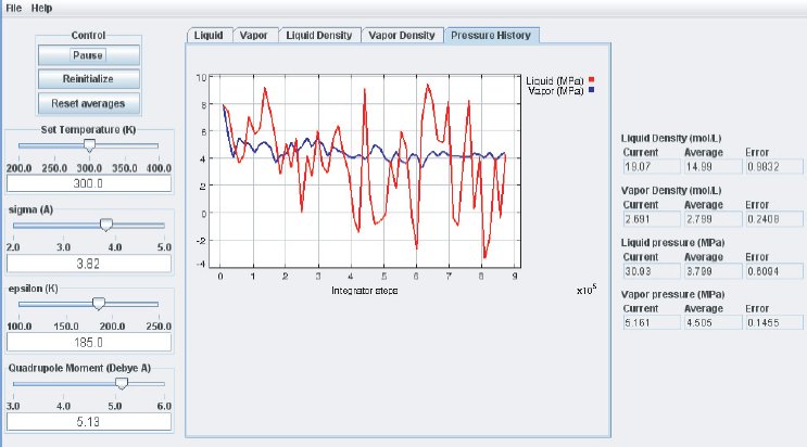
Set the simulation parameters to :

Set Temperature to 300 K
Set $\sigma$ to 3.82
Set $\varepsilon$ to 185 K
Set the Quadrupole moment to 5.13 debye $\cdot$ Å

Start the simulation by pushing the Start button. The button will change its label to “Pause” which can be used to pause and continue the simulation at any given time.

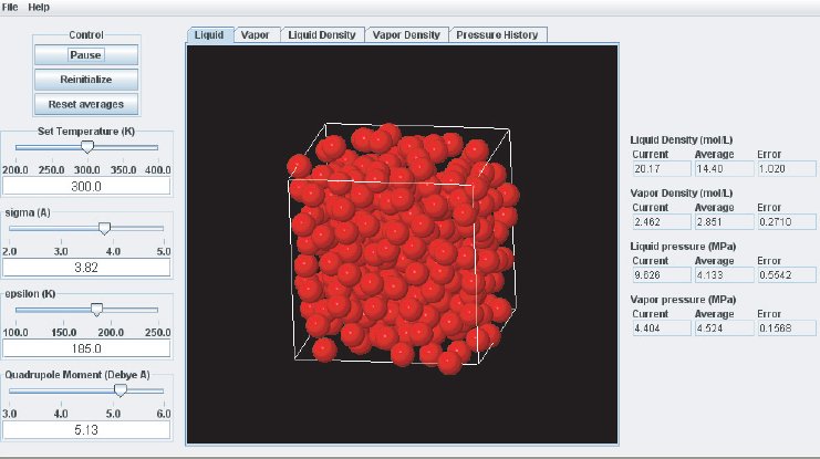
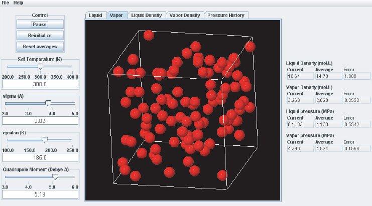
As the simulation proceeds, observe the atoms in the two phases. Below the critical point, the liquid phase will change to look more like what one would expect: atoms sticking close together. At the same time, the gas phase configuration becomes more “dilute” which is also expected for a system well below its critical point. This behavior can also me monitored in the density plots where we typically see the density in the liquid increase and the density in the gas phase drop. The total volume, i.e. the combined volumes of the vapor and liquid phases, is kept constant (similar to an experiment where the VLE is measured isochorically). Because of the changing numbers of atoms the pressures in the two phases adjust accordingly, which can be observed in the “Pressure History” plot tab and also in the running averages in the Data Display panel.

When the simulation is started the oscillations in the properties will be large because the initial state of the system is far from equilibrium. To monitor the average pressures it is best to press the “Reset Averages” button after the initial $10^6$ integrator steps. This will keep the simulation running but it will reset the plots and the data collection for the averages will start freshly from the current integrator step. The “Error” printed for each property in the data Panel is the statistical error of the running average; it does not necessarily indicate if the results are converged. For example, there might be a steady drift in the vapor density despite small magnitudes of the Vapor Density Error listed in the Data Display Panel. Below are some screen shots showing what a simulation typically looks like after roughly $10^6$ steps, and what data the various plots contain:

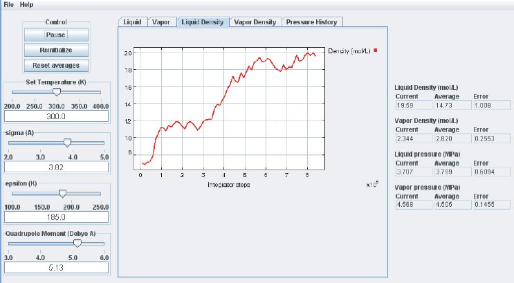
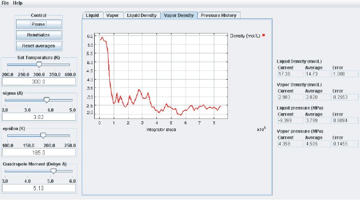
It takes approximately $10^6$ integration steps (roughly 10 to 20 min on a modern (2008 vintage) PC) for the most drastic variations in the properties to disappear. Press the “Reset averages” button after the first million integrator steps. From then on keep monitoring the averages for about $10^7$ integrator steps. This will take up to a few hrs on a modern PC. Use more steps if necessary to diminish statistical errors in the computed properties and to make sure there are no systematic drifts in the calculated properties (this is easily revealed by the various plots). You will find that the vapor pressure and the liquid density converge rather quickly at temperatures well below the critical point, but that the density of the vapor and the pressure in the liquid take many integrator steps to converge. Negative pressures for the liquid phase are not uncommon for earlier stages of the simulation; the unphysical value simply indicates that the average has not yet converged. Check the magnitude of the oscillations in the various plots compared to the value of the average. For the pressure in the liquid, the oscillations are typically very large and it takes many steps for the average to become meaningful.

Eventually, the pressures in the liquid and vapor phase will become very similar which indicates that the simulation is converging. The pressures will not become identical, as they ideally should, because of some approximations made in the computation. They should be equal to within the errors printed. Upon convergence of the simulation, we have found the pressure P corresponding to the selected temperature T for the vapor–liquid equilibrium. Therefore, we have calculated one (P, T) point of the vapor–liquid coexistence curve in the phase diagram of the substance described by the inter–molecular potential parameters used for the simulation.